The Reuters Dataset contains a set of short newswires and their topics, published by Reuters in 1986. Each topic has at least 10 examples in the training set. Our job is to classify Reuters newswires into 46 different mutually exclusive topics. There are 8982 training examples and 2246 testing examples.
Code
library(keras)reuters =dataset_reuters(num_words =10000) # 10,000 most frequently occurring wordsc(c(train_data, train_labels), c(test_data,test_labels)) %<-% reuterstrain_labels[[1]] # label associated with an example is an integer between 0 and 45 - a topic indextest_labels[[1]] # 1st test label is a topic index of 3 - we will predict this later
To vectorize labels, there are two possibilities : (1) cast the label list as an integer tensor (2) One-hot encoding.
One-hot encoding is a widely used format for categorical data, also called categorical encoding. Here, one-hot encoding of the labels consists of embedding each label as an all-zero vector with a 1 in the place of the label index.
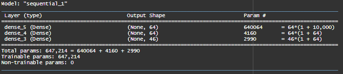
Here we are dealing with output which has 46 classes i.e. the dimensionality of output space is much larger. Earlier there were 2 classes.
In a stack of dense layers, each layer can only access information present in the output of the previous layer. If one layer drops some information relevant to the classification problem, this information can never be recovered by later layers: each layer can potentially become an information bottleneck. In the previous e.g. we used 16-dimensional intermediate layers, but a 16-dimensional space may be too limited to learn to separate 46 different classes; such small layers may act as information bottlenecks, permanently dropping relevant information.
We end the network with a dense layer of size 46 because we have to classify into 46 different classes. The use of softmax activation means that the network will output a probability distribution over the 46 different output classes.
Compile
Code
model %>%compile(optimizer="rmsprop",loss="categorical_crossentropy",metrics=c("accuracy"))
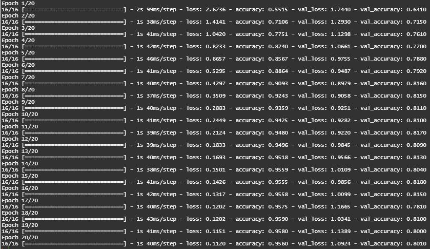
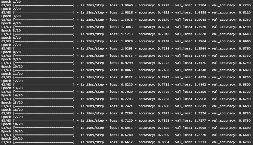
history = model %>%fit(partial_x_train, partial_y_train, epochs=20,batch_size=512,validation_data=list(x_val, y_val))
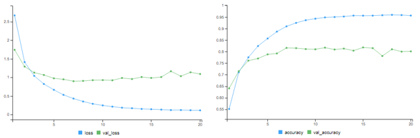
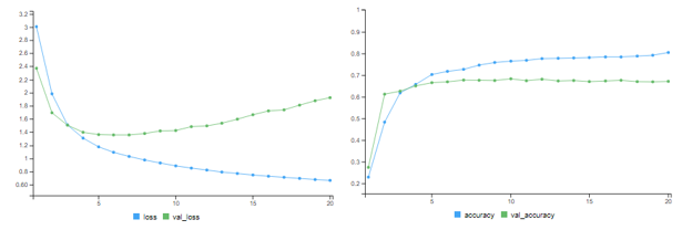
Figure : Training Logs
The network begins to overfit after 9 epochs !
Code
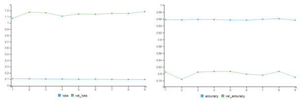
# change epochs to 9history = model %>%fit(partial_x_train, partial_y_train, epochs=9, batch_size=512,validation_data =list(x_val, y_val))# training accuracy = 96.64% # validation accuracy = 79%results = model %>%evaluate(x_test, one_hot_test_labels) # test accuracy = 78.54%
Accuracy around 78-79%. In case of a balanced binary classification problem, the accuracy reached by a purely random classifier would be 50%
Code
# Purely Random Classifiertest_labels_copy = test_labelstest_labels_copy =sample(test_labels_copy)length(which(test_labels==test_labels_copy))/length(test_labels) # 18%
But in this case it’s closer to 18%, so the results seem pretty good, at least when compared to a random-baseline.
Predictions
Code
predictions = model %>%predict(x_test)dim(predictions) # 2246 46# returns a probability distribution over all 46 topics thus vector of # length 46 for all 2246 test exampleswhich.max(predictions[1,]) # 4# class with highest probability is '4' - as we saw above, # the actual topic index is 3predictions[1,4]# topic index 4 is predicted with a probability of 98.499%predictions[1,3]# topic index 3 is predicted with a probability of 0.0001%
The network peaks at 71% validation accuracy i.e. 8% absolute drop - mostly due to the fact that we’re trying to compress a lot of information into an intermediate space that is too low-dimensional. The network is able to cram most of the necessary information into these 8-dimensional representations, but not all of it.